A collaboration between Lewis McLain & AI

It was my last semester in the Business School at UNT. I majored in Accounting, but my true love was Cost Accounting. I was the only student at the time to have taken three courses in the subject as they phased out one course and substituted another. I had become intrigued with Fortran a few semesters earlier. Then I was introduced to the use of simultaneous equations for cost allocations. We had to hand calculate the math; therefore, the number of departments was unrealistically small. Professor Nelson would bring his loud but amusing “peanut thrasher,” like the one below, to show us the arithmetic behind the linear algebra equations. Remember, this was 1971 and the first electronic calculators were just being introduced.

After graduation, I started at Garland as the first Budget Director there. Early in my 5-year tenure, my interest turned to a cost allocation study conducted by one of the then-Big 8 accounting firms: Ernst & Ernst. All I had was a hard copy, but the firm had done a decent job of explaining the step-down methodology for allocating indirect costs to direct service departments. I married my Fortran skills to my cost accounting love and reproduced every number in the report, including all internal calculations that weren’t fully shown in the report.

A few years later, when I had a consulting firm of my own, cost allocation plans were the hot ticket. Guiding my staff, we produced an example of cost allocation using simultaneous equations, leveraging features built into Lotus 1-2-3. We even met with HUD in Fort Worth to demonstrate and to get approval to use that methodology.

Excel has improved features to conduct allocations using simultaneous equations. This paper is to provide both examples and an actual Excel spreadsheet to illustrate this approach.

Introduction

Every public organization depends on a set of indirect (support) departments to keep operations running: Finance, HR, IT, Procurement, Central Services, Legal, Facilities, Fleet, and more. Yet the costs of these support functions do not exist for their own sake—they exist because frontline departments depend on them to deliver police protection, fire response, public works operations, community services, transit, parks, library services, public health, and housing.

For budgeting, grant reimbursement, user fees, performance management, and internal accountability, cities must determine how much of each support department’s cost should be assigned to the frontline operating units.

This process is known as cost allocation.

Over time, several methodologies have evolved—from the simple and intuitive to the complex but mathematically precise. This essay summarizes those methods, shows why they differ, and explains why the reciprocal (simultaneous equations) method is the single most accurate approach for modern governments—particularly now that Excel and AI make it practical for any city.

⭐ I. Comparative Overview of Cost Allocation Methods

1. Direct Allocation Method

The simplest method assigns each indirect cost pool to direct departments usually based only on one driver (e.g., HR allocated by FTEs).
Strength: Easy and transparent.
Weakness: Ignores the fact that indirect departments often support each other.

Example problem:

• HR supports IT
• IT supports HR
  Direct step-down allocation ignores this two-way relationship.

2. Single Step-Down Method

This sequential method assigns indirect departments in a fixed order:

1. Choose an indirect department (like Finance).
2. Allocate its cost to all departments (including other indirects).
3. “Close” Finance.
4. Move to the next indirect department.

Strength:

• Still simple and widely used.

Weakness:

• The order of allocation matters.
• Ignores most reciprocal support.
• Can distort results significantly.
• Can be scrutinized by external organizations like Wholesale Water Customers or Customer Cities like Transit Agencies.

3. Double Step-Down Method

A refinement to capture stronger two-way interaction between the first two indirect departments before the regular single step-down sequence.

Strength:

• Captures limited reciprocal flows.
• Still Excel-friendly.

Weakness:

• Only partially improves accuracy.
• Still depends heavily on order.

4. Multiple Iteration Method (Iterative Step-Down)

Run the step-down sequence many times until changes become small.

Strength:

• Approximates reciprocal flows more closely.

Weakness:

• Still an approximation.
• Not guaranteed to converge.
• Harder to audit.
• Still not exact.

⭐ II. The Reciprocal (Simultaneous Equations) Method

The reciprocal method recognizes the full truth: indirect departments support each other in complex, circular ways.

Examples:

• IT supports Finance, but Finance supports IT.
• Facilities supports every department, including those that support Facilities.
• Administration supports Legal, Legal supports Administration.

These interactions create a system of simultaneous linear equations.

Traditionally, this method required advanced math or expensive software. Today, Excel’s MINVERSE() and MMULT() functions, combined with transparent model structure, make the reciprocal method practical and accessible. Hint: don’t worry about higher mathematics too much at this point. Remember that Excel is going to take care of all that work for us.

Definition:

$$A \cdot X = B$$Where:

• A = reciprocal system matrix = (Identity – Wssᵀ)
• X = fully loaded indirect cost vector
• B = initial indirect budgets

Solution:$$X = (A^{-1}) B$$X=(A−1)B

This produces the exact full cost of each indirect department after capturing all circular support flows.

⭐ III. Federal Recognition & Regulatory Alignment

Federal agencies have long endorsed this approach.

OMB Uniform Guidance (2 CFR 200)

Defines indirect costs and requires that they be allocated based on:

“relative benefits received.”
— 2 CFR 200.405(d)

The reciprocal method is the only method that fully meets this standard when indirect departments support each other.

ASMB C-10 (HHS Implementation Guide)

States that the cost allocation principles include:

“…guidance for interpretation and implementation…”
— ASMB C-10, Preface

The examples illustrate precisely the type of reciprocal circularity the method captures.

Consulting Industry

Large national firms implementing federal cost plans (e.g., Maximus, MGT, Guidehouse, Plante Moran, BerryDunn) have used reciprocal methods for:

• Statewide cost allocation plans (SWCAP)
• Department-level indirect cost plans
• Federal indirect rate proposals
• Research F&A rate determination
• Public safety overhead models
• Public works cost-of-service studies

The reciprocal method is the recognized gold standard.

⭐ IV. Why the Reciprocal Method Is Superior

✔ 1. Accurate

Captures all reciprocal flows between indirect departments.

✔ 2. Order-independent

Step-down methods depend on sequencing.
Reciprocal method always returns the same answer.

✔ 3. Auditable

Every stage is transparent and traceable:

• raw drivers
• normalized weights
• allocation matrices
• fully loaded indirects
• final allocations

✔ 4. Complies with Federal Standards

Directly aligns with “relative benefits received.”

✔ 5. Excel now makes it easy

One formula computes the X vector:

=MMULT(MINVERSE(A), B)

✔ 6. AI eliminates complexity

AI can:

• Build matrices
• Check formulas
• Validate sums
• Ensure consistency
• Explain model steps

This allows smaller governments to use the same rigor once reserved for big agencies.

⭐ V. How This Model Is Built — A Practical Walkthrough

Your accompanying spreadsheet (now fully dynamic) uses the exact full reciprocal process in 10 clear, auditable steps, each mapped to a tab.

Below is the Technical Appendix rewritten to match those tabs exactly.

⭐ TECHNICAL APPENDIX — TAB-BY-TAB GUIDE TO THE MODEL

This Appendix mirrors the spreadsheet structure so users can follow the math end-to-end.

📘 Step 0 — Raw Metrics (Scaled)

Input tab.

Contains operational drivers:

• FTEs
• Devices
• Budget (scaled to $10M total for interpretability)
• SqFt
• Vehicles
• Procurement counts
• Legal hours
• Records
• Risk claims

These raw values determine how indirect departments distribute their services across the full organization.

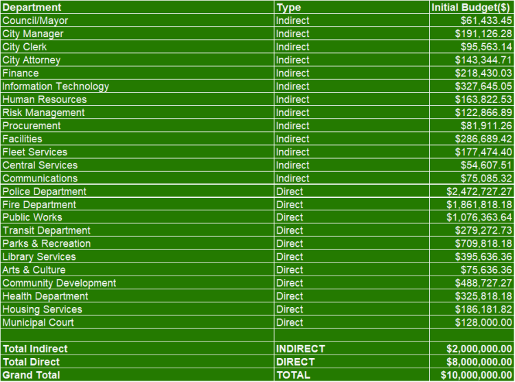
📘 Step 1 — Initial Budgets

Financial inputs only.

• $2,000,000 indirect
• $8,000,000 direct
• $10,000,000 total (model base)

These do not equal Step 0 totals.
Step 0 contains drivers, some of which might be financial budgets or components of same.

📘 Step 2 — Drivers_Norm

Dynamic calculations.

For each indirect department:

• Identify driver (Budget, FTEs, Devices, etc.)
• Normalize each department’s driver value by the total driver column
• Each row sums to 1.0

These normalized weights feed the W matrix. Normalization means taking the raw driver numbers—like FTEs, devices, or square footage—and expressing each one as part of the whole. Each department’s value becomes its percentage share of the total.

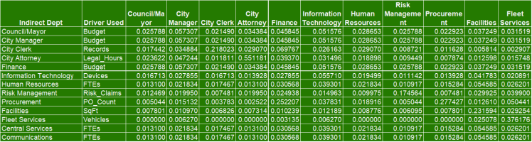
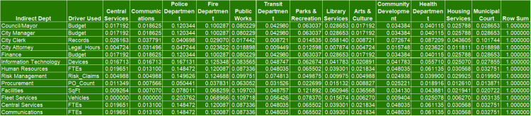
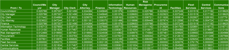
📘 Step 3 — W Matrix

Dynamic.

The full allocation matrix:

• Rows = indirect departments
• Columns = all departments
• Values = proportions from Step 2
• Row sums = 1.0

This matrix determines how indirect departments allocate their costs.

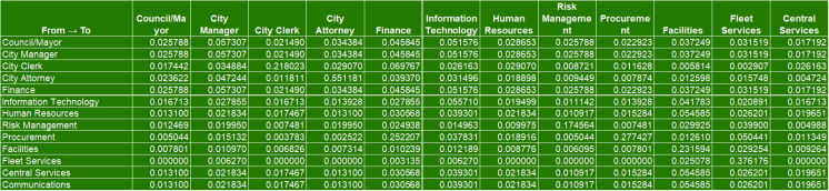
📘 Step 4 — Wss (Indirect→Indirect)

Dynamic.

Extracts the top-left 13×13 block of W:

• Shows reciprocal flows between indirect departments
• Inputs to the reciprocal system matrix A

📘 Step 5 — A Matrix

Dynamic.$$A = I – Wss^{T}$$A=I−WssT

Where:

• I = identity matrix
• Wssᵀ = transpose of indirect block

Diagonal entries show remaining self-load.
Off-diagonals show cross-support.

📘 Step 6 — B Vector

Dynamic.

Pulls the initial indirect budgets from Step 1.

This is the starting point for the reciprocal solution.

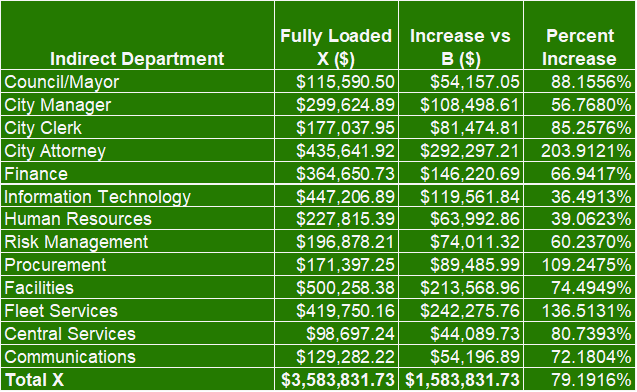
📘 Step 7 — X Vector

Dynamic and computed via Excel matrix algebra.$$X = A^{-1} B$$X=A−1B

These are the fully loaded indirect costs after accounting for:

• mutual support
• circular relationships
• internal cost absorption

Sum(X) ≈ Sum(B).

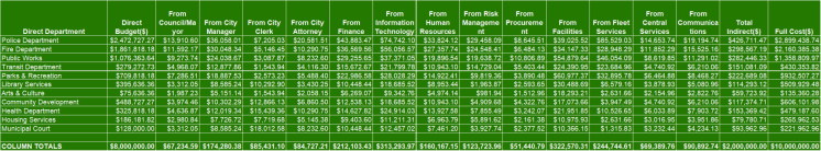
📘 Step 8 — Allocation to Direct Departments

Dynamic allocation of fully loaded indirects.

Uses the formula:$$\text{Allocated}_{i \to j} = X_i \cdot W_{i,j}$$Allocatedi→j​=Xi​⋅Wi,j​

Where:

• i = indirect dept
• j = direct dept

This produces the overhead assigned to each operating unit.

Final columns:

• Total Indirect
• Full Cost = Direct Budget + Indirect Assigned

📘 Step 9 — Summary (Full Cost)

Dynamic.

Shows for each direct department:

• Direct Budget
• Indirect Allocated
• Full Cost
• Percent Increase
• Percent of Total

Full costs sum to $10,000,000.

📘 Step 10 — Totals Check

Dynamic validation.

Shows:

• Total Before = $10,000,000
• Total After = $10,000,000
• Difference = 0

Confirms mathematical integrity.

This demonstrates:

• No cost drift
• No rounding loss
• No double-counting
• Reciprocal method implemented correctly

⭐ Conclusion

Thanks to the maturity of spreadsheet functions and the availability of AI-driven guidance, the reciprocal method—once limited to large consulting firms and federal cost plans—is now achievable for any city with Excel.

This model provides:

• Accuracy
• Transparency
• Regulatory alignment
• Audit readiness
• Dynamic recalculation
• Clear documentation

It ensures that each department’s cost truly reflects the full resources required to serve the public.

Permission is granted for you to share this model with any other governmental entity, with attribution, please.